2. The Simulator General Use
The following section describes the first steps to use the Gridsim simulator and its built-in modules.
Currently, the simulator provides:
- Global simulation
- Electrical simulation
- Cyber-physical simulation
- Thermal simulation
- Control of simulation elements
- Record of simulation elements
2.1. Simulation
2.1.1. Global simulation
Module author: Gillian Basso <gillian.basso@hevs.ch>
Code author: Michael Clausen <clm@hevs.ch>
The gridsim.simulation module defines a simple way to access to the
simulator and offers interfaces of communication with users.
To create a new gridsim simulation you have to initialize a Simulator
object. Then you will use the different simulation modules in order to define
the electrical and/or thermal topology and parametrize the data recorders and
controllers to form the complete simulation.
Once done, you should always start with a reset to ensure that all simulation
elements are in a defined state. Then you can either do a simple step using the
method Simulator.step() or run a simulation until a given time with a
given step size using the method Simulator.run().
Example:
from gridsim.unit import units
from gridsim.simulation import Simulator

# Create the main simulator object.
sim = Simulator()

# Build topology using the different simulation modules
...

# Run the simulation from the
sim.run(1*units.hours, 100*units.milliseconds)
As Gridsim is based on modules. You can get access to the simulation modules by using special attributes of the core simulation object:
sim = Simulation()
sim.<module_name>
So if you import for example gridsim.electrical, you can get the
simulation module by typing:
sim = Simulator()
el = sim.electrical
Note
Actually, the name of the module is the returned value of
gridsim.core.AbstractSimulationModule.attribute_name().
Refer to the module you want to use to retrieve the module name.
-
class
gridsim.simulation.Recorder(self, attribute_name, x_unit=None, y_unit=None)¶ Bases:
objectDefines the interface an object has to implement in order to get notified between simulation steps with a reference to the observed object, the name of the attribute/property, the actual time and the actual value of the observed attribute/property.
To add a recorder to the simulation, use
Simulator.record().Parameters: - attribute_name (str) – The name of the attribute observed by this recorder.
- x_unit (type or unit see
gridsim.unit) – The unit of the horizontal axis - y_unit (type or unit see
gridsim.unit) – The unit of the vertical axis
-
attribute_name¶ The name of the attribute observed by this recorder.
-
on_simulation_reset(self, subjects)¶ This method is called by the simulation on order to inform the recorder that the simulation has been reset. The parameter
subjectsis a list of all subjects that are observer by the actual recorder. The method is called for each binding the recorder has with the simulation. This means that you do 3 calls toSimulator.record()with the same recorder, this method is called 3 times.Parameters: subjects (list or tuple of gridsim.core.AbstractSimulationElement) – list of all observed objects.
-
on_simulation_step(self, time)¶ This method is called each time the simulation just completed a step. This method is optional and not required to re-implement a recorder.
Parameters: time (time, see gridsim.unit) – The actual simulation time.
-
on_observed_value(self, subject, time, value)¶ Called by the main simulation engine between each simulation step in order the recorder can save the time-value pair of one or multiple
AbstractSimulationElementsubclass(es). Any recorder is required to implement this method.Parameters: - subject (
AbstractSimulationElement) – The object that will be observed by the recorder. - time (time, see
gridsim.unit) – The actual time of the simulation. - value (Depends attribute...) – The actual value of the attribute/property of the subject.
- subject (
-
class
gridsim.simulation.Simulator(self)¶ Bases:
objectGridsim main simulation class. Moves the simulation of all modules on in time and groups all simulation modules. The constructor creates automatically an instance of each registered simulation module. The fact to import a simulation module to the user’s project registers the module automatically within the main simulation class. So only modules really used by the simulation are instantiated.
-
static
register_simulation_module(module_class)¶ Registers a simulation module class within the main simulator class. Note that you register the class, the simulator automatically instantiates an object of the class in its own constructor every time an instance of the simulator is created.
Parameters: module_class ( gridsim.core.AbstractSimulationModule) – The class to register as a simulation module.
-
find(self, module=None, uid=None, friendly_name=None, element_class=None, instance_of=None, has_attribute=None, close_to=None)¶ Finds all
AbstractSimulationElementderived objects matching the given criteria by searching on either the given Gridsim simulation module or by searching the whole simulation of the module was not specified. Note that the method returns always a list of element, even if only a single instance is found. All parameters are optional, iffind()will be called without any parameters, the list of all element in the actual simulation will be returned.Parameters: - module (str) – The module to search for element.
- uid (int) – ID of the element. Note that these ID’s are only unique for a given class inside a module, so you should never search just for an ID without specifying either the class or at least the module.
- friendly_name (str) – The friendly name to search for.
- element_class (type) – The exact class the element has to be an instance of. Superclasses are not considered.
- instance_of (type) – The object has to be an instance of the given class, whereas this can be the superclass of the object too.
- has_attribute (str) – The object should have an attribute with the given
name. This can be used in order to find all objects that have a
powerattribute. - close_to ((Position, float)) – The object’s position should be closer to the given one than the given radius. The parameters should be passed as tuple of the position and the radius in meters [m]
Returns: List of
AbstractSimulationElementmatching the given criteria.Example:
from gridsim.util import Position
from gridsim.simulation import Simulator
from gridsim.electrical.core import AbstractElectricalCPSElement
from gridsim.electrical.network import ElectricalSlackBus
from gridsim.thermal.element import ThermalProcess

# Create the simulation.
sim = Simulator()

# Here you could create the topology of the actual simulation...
# ...

# Get all elements of the electrical simulation module
#   (Both statements do exactly the same).
print sim.find(module='electrical')
print sim.electrical.find()

# Get the electrical slack bus.
print sim.electrical.find(element_class=ElectricalSlackBus)

# Get all electrical consumer/producer/storage elements.
print sim.electrical.find(instance_of=AbstractElectricalCPSElement)

# Get the element with friendly name 'bus23'.
print sim.find(friendly_name='bus23')

# Get all elements which have the 'temperature' attribute.
print sim.find(has_attribute='temperature')

# Get all elements of the simulation that are close (1km)
#   to a given point (Route du rawyl 47, Sion).
print sim.find(close_to=(Position(46.240301, 7.358394, 566), 1000))

# Of course these search criteria can be mixed.
#   For example we search the 5th thermal process.
print sim.find(module='thermal', element_class=ThermalProcess, uid=5)
-
reset(self, initial_time=0*units.second)¶ Resets (re-initializes) the simulation.
Parameters: initial_time (time, see gridsim.unit) – The initial time from which the simulation starts. Defaults to0.
-
step(self, delta_time)¶ Executes a single simulation step on all modules.
Parameters: delta_time (time, see gridsim.unit) – The delta time for the single step.
-
run(self, run_time, delta_time)¶ Runs the simulation for a given time.
The run_time parameter defines the duration the simulation has to run. If a simulation was already run before, the additional duration is run in addition.
Parameters: - run_time (time, see
gridsim.unit) – Total run time. - delta_time (time, see
gridsim.unit) – Time interval for the simulation.
- run_time (time, see
-
record(self, recorder, subjects, conversion=None)¶ Adds a recorder to an attribute of an object. The recorder has to implement the
Recorderinterface in order to receive the data of the given attribute after each simulation step.Parameters: - recorder (
Recorder) – Reference to the recorder object. This object gets notified about the changes of the object’s attribute at each simulation step. - subjects (list or tuple of
AbstractSimulationElement) – The subjects of the recorder, in other words the objects which is attributes has to be recorded. If None, the time is the only one value recorded, withon_simulation_step(). - conversion (lambda context) –
Lambda function to convert the actual value taken from the attribute before recording. The lambda function gets a single parameter
contextwhich is a named tuple with the following element:value: The actual value just read from the simulation element’s attribute.
time: The actual simulation time.
delta_time: The time step just simulated before updating the recorder. This can be handy in order to calculate for example the power of a delta-energy value.
Returns: Reference to the recoder.
- recorder (
-
static
2.1.2. Electrical simulation
Module author: Gilbert Maitre <gilbert.maitre@hevs.ch>
The gridsim.electrical module implements the electrical part of the
gridsim simulator. It basically manages Consuming-Producing-Storing (CPS)
Elements, which consume (positive sign) and/or produce (negative sign) a
certain amount of energy (delta_energy) at each simulation step.
CPS elements may be attach to buses of an electrical power network, which is also made of branches as connections between buses.
Example:
1 2 3 4 5 6 7 8 9 10 11 12 13 14 15 16 17 18 19 20 21 22 23 24 25 26 27 28 29 30 31 32 33 34 35 36 37 38 39 40 41 42 43 44 45 46 47 48 49 50 51 52 53 54 55 56 57 58 59 60 61 62 63 64 65 66 67 68 69 70 71 72 73 74 75 76 77 78 79 80 | from gridsim.simulation import Simulator
from gridsim.unit import units
from gridsim.electrical.network import ElectricalPVBus, ElectricalPQBus,\
ElectricalTransmissionLine, ElectricalGenTransformer
from gridsim.electrical.element import GaussianRandomElectricalCPSElement, \
ConstantElectricalCPSElement
from gridsim.recorder import PlotRecorder
from gridsim.electrical.loadflow import DirectLoadFlowCalculator
from gridsim.iodata.output import FigureSaver
# Create the simulation.
sim = Simulator()
esim = sim.electrical
esim.load_flow_calculator = DirectLoadFlowCalculator()
# add buses to simulator
# slack bus has been automatically added
esim.add(ElectricalPQBus('Bus 1'))
esim.add(ElectricalPQBus('Bus 2'))
esim.add(ElectricalPQBus('Bus 3'))
esim.add(ElectricalPVBus('Bus 4'))
# add branches to simulator
# this operation directly connects them to buses, buses have to be already added
# variant 1
esim.connect('Branch 5-3', esim.bus('Slack Bus'), esim.bus('Bus 3'),
ElectricalGenTransformer('Tap 1', complex(1.05), 0.03*units.ohm))
tl1 = esim.connect('Branch 3-1', esim.bus('Bus 3'), esim.bus('Bus 1'),
ElectricalTransmissionLine('Line 1',
1.0*units.metre,
0.35*units.ohm, 0.1*units.ohm))
tl2 = esim.connect('Branch 3-2', esim.bus('Bus 3'), esim.bus('Bus 2'),
ElectricalTransmissionLine('Line 2',
1.0*units.metre,
0.3*units.ohm, 0.08*units.ohm,
2*0.25*units.siemens))
tl3 = esim.connect('Branch 1-2', esim.bus('Bus 1'), esim.bus('Bus 2'),
ElectricalTransmissionLine('Line 3',
1.0*units.metre,
0.25*units.ohm, 0.04*units.ohm,
2*0.25*units.siemens))
esim.connect('Branch 4-2', esim.bus('Bus 4'), esim.bus('Bus 2'),
ElectricalGenTransformer('Tap 2', complex(1.05), 0.015*units.ohm))
# attach electrical elements to buses, electrical elements are automatically
# added to simulator
esim.attach('Bus 1', GaussianRandomElectricalCPSElement('Load1',
1.6*units.watt, 0.1*units.watt))
esim.attach('Bus 2', GaussianRandomElectricalCPSElement('Load2',
2.0*units.watt, 0.2*units.watt))
esim.attach('Bus 3', GaussianRandomElectricalCPSElement('Load3',
3.7*units.watt, 0.3*units.watt))
esim.attach('Bus 4', ConstantElectricalCPSElement('Gen', -5.0*units.watt))
# Create a plot recorder which records power on each bus.
bus_pwr = PlotRecorder('P', units.second, units.watt)
sim.record(bus_pwr, esim.find(element_class=ElectricalPQBus))
# Create a plot recorder which records power on transmission lines.
line_pwr = PlotRecorder('Pij', units.second, units.watt)
sim.record(line_pwr, [tl1, tl2, tl3])
# It is recommended to perform the simulator reset operation.
sim.reset()
print("Running simulation...")
# Run the simulation for two hours with a resolution of 1 minute.
total_time = 2*units.hours
delta_time = 1*units.minutes
sim.run(total_time, delta_time)
print("Saving data...")
# Save the figures as images.
saver = FigureSaver(bus_pwr, "PQ Bus power")
saver.save('./output/bus_pwr.pdf')
saver = FigureSaver(line_pwr, "Line power")
saver.save('./output/line_pwr.pdf')
|
shows a pure electrical example made of a reference 5-bus network (see e.g. Xi-Fan Wang, Yonghua Song, Malcolm Irving, Modern power systems analysis), to the non-slack buses of which are attached 4 CPS elements : 1 with constant power, production, 3 with random gaussian distributed power consumption.
Here is the class diagram of the electrical package:

2.1.2.1. Electrical package
Module author: Gillian Basso <gillian.basso@hevs.ch>
Code author: Gilbert Maitre <gilbert.maitre@hevs.ch>
-
class
gridsim.electrical.simulation.ElectricalSimulator(*args, **keywords)¶ Bases:
gridsim.core.AbstractSimulationModuleGridsim main simulation class for electrical part. This module is automatically added to the
Simulatorwhen importing any class or module ofgridsim.electricalpackage.To access this class from simulation, use
Simulatoras follow:# Create the simulation. sim = Simulator() esim = sim.electrical
Parameters: calculator ( AbstractElectricalLoadFlowCalculator) – The load flow calculator used by the simulator-
load_flow_calculator¶ The load flow calculator
See also
gridsim.electrical.loadflowfor more details.
-
add(self, element)¶ Add the element to the electrical simulation but do not connect it with other element. use other functions such as
connect()andattach()to really use the element in the simulation.Parameters: element ( AbstractElectricalElement) – the element to addReturns: the given element
-
bus(self, id_or_friendly_name)¶ Retrieves the bus with the given id or friendly name.
Parameters: id_or_friendly_name ((int, str)) – the identifier of the bus
Returns: the
ElectricalBusRaises: - KeyError – if the friendly name is not valid
- IndexError – if the id is not valid
-
branch(self, id_or_friendly_name)¶ Retrieves the branch with the given id or friendly name.
Parameters: id_or_friendly_name ((int, str)) – the identifier of the bus
Returns: Raises: - KeyError – if the friendly name is not valid
- IndexError – if the id is not valid
-
cps_element(self, id_or_friendly_name)¶ Retrieves the branch with the given id or friendly name.
Parameters: id_or_friendly_name ((int, str)) – the identifier of the bus
Returns: Raises: - KeyError – if the friendly name is not valid
- IndexError – if the id is not valid
-
connect(self, friendly_name, bus_a, bus_b, two_port)¶ Creates a
ElectricalNetworkBranchwith the given parameters and adds it to the simulation.See also
Parameters: - friendly_name (str) – the name of the branch
- bus_a (
ElectricalBus) – the first bus the branch connects - bus_b (
ElectricalBus) – the second bus the branch connects - two_port – the element placed on the branch
Returns: the new
ElectricalNetworkBranch
-
attach(self, bus, el)¶ Attaches the given bus to the given element. After this function, the element is present in the simulation and will provide electrical energy to the simulation
Parameters: - bus (
ElectricalBus) – the bus the element has to be attached - el (
AbstractElectricalCPSElement) – the new element of the simulation
- bus (
-
attribute_name(self)¶ Returns the name of this module. This name is used to access to this electrical simulator from the
Simulator:# Create the simulation. sim = Simulator() esim = sim.electrical
Returns: ‘electrical’ Return type: str
-
all_elements(self)¶ Returns a list of all
AbstractElectricalElementcontained in the module. The core simulator will use these lists in order to be able to retrieve objects or list of objects by certain criteria usinggridsim.simulation.Simulator.find().
-
reset(self)¶ Calls
gridsim.core.AbstractSimulationElement.reset()of each element in this electrical simulator, added by theElectricalSimulator.add().
-
calculate(self, time, delta_time)¶ Calls
gridsim.core.AbstractSimulationElement.calculate()of eachAbstractElectricalCPSElementin this electrical simulator, added by theElectricalSimulator.add().Parameters: - time (int or float in second) – The actual simulation time.
- delta_time (int or float in second) – The time period for which the calculation has to be done.
-
update(self, time, delta_time)¶ Updates the data of each
AbstractElectricalCPSElementin this electrical simulator added by theElectricalSimulator.add()and calculate the load flow withAbstractElectricalLoadFlowCalculator.Parameters: - time (int or float in second) – The actual simulation time.
- delta_time (int or float in second) – The time period for which the calculation has to be done.
-
2.1.2.2. Electrical load flow
Module author: Michael Sequeira Carvalho <michael.sequeira@hevs.ch>
Module author: Gilbert Maitre <gilbert.maitre@hevs.ch>
Code author: Gilbert Maitre <gilbert.maitre@hevs.ch>
This module provides a toolbox to Gridsim to perform computation of electrical values within the electrical network, in other words to solve the so-called power-flow problem:
-
class
gridsim.electrical.loadflow.AbstractElectricalLoadFlowCalculator(self)¶ Bases:
objectThis class is the base for all calculator that have been or are going to be implemented to solve the power-flow problem.
At initialization the user has to give the reference power value s_base (all power values are then given relative to this reference value), the reference voltage value v_base (all voltage values are then given relative to this reference value), a boolean array is_PV specifying which one among the buses is a
ElectricalPVBus(the bus with 1st position is slack, the others nonElectricalPVBusareElectricalPQBus), an integer array b specifying for each branch the bus id it is starting from and the bus id it is going to, a complex array Yb specifying admittances of each network branch.-
s_base= None¶ The reference power value. Set by
AbstractElectricalLoadFlowCalculator.update()
-
v_base= None¶ The reference voltage value. Set by
AbstractElectricalLoadFlowCalculator.update()
-
update(self, s_base, v_base, is_PV, b, Yb)¶ Updates values of the calculator.
Parameters: - s_base (float) – reference power value
- v_base (float) – reference voltage value
- is_PV (1-dimensional numpy array of boolean) – N-long vector specifying which bus is of type
ElectricalPVBus, where N is the number of buses including slack. - b (2-dimensional numpy array of int) – Mx2 table containing for each branch the ids of start and end buses.
- Yb (2-dimensional numpy array of complex) – Mx4 table containing the admittances Yii, Yij, Yjj, and Yji of each branch.
-
calculate(self, P, Q, V, Th, scaled)¶ Compute all bus electrical values determined by the network:
- takes as input active powers P of all non-slack buses, reactive powers
of
ElectricalPQBusand voltage amplitudes ofElectricalPVBus; all these values have to be placed by the user at the right place in the N-long vectors, P, Q, and, respectively, V, passed to this method. - outputs active power of slack bus, reactive powers of
ElectricalPVBus, voltage amplitudes ofElectricalPQBus, and voltage angles of all buses; all these values are placed by this method at the right place in the N-long vectors P, Q, V, and, respectively, Th, passed to this method.
Parameters: - P (1-dimensional numpy array of float) – N-long vector of bus active powers, where N is the number of buses including slack.
- Q (1-dimensional numpy array of float) – N-long vector of bus reactive powers, where N is the number of buses including slack.
- V (1-dimensional numpy array of float) – N-long vector of bus voltage amplitudes, where N is the number of buses including slack.
- Th (1-dimensional numpy array of float) – N-long vector of bus voltage angles, where N is the number of buses including slack.
- scaled (boolean) – specifies whether electrical input values are scaled or not
Returns: modified [P, Q, V, Th]
Return type: a list of 4 element
- takes as input active powers P of all non-slack buses, reactive powers
of
-
get_branch_power_flows(self, scaled)¶ Compute all branch power flows. Cannot be called before method
AbstractElectricalLoadFlowCalculator.calculate(). Returns a tuple made of 4 1-dimensional numpy arrays:- Pij containing branch input active powers,
- Qij containing branch input reactive powers,
- Pji containing branch output active powers,
- Qji containing branch output reactive powers.
Parameters: scaled (boolean) – specifies whether output power flows have to be scaled or not Returns: 4 M-long vector, where M is the number of branches Pij: vector of active powers entering the branch from the from-bus termination Qij: vector of reactive powers entering the branch from the from-bus termination Pji: vector of active powers entering the branch from the to-bus termination Qji: vector of reactive powers entering the branch from the to-bus termination Return type: tuple of one-dimensional numpy arrays of float
-
get_branch_max_currents(self, scaled)¶ Compute the maximal current amplitude of each branch. Cannot be called before method
AbstractElectricalLoadFlowCalculator.calculate(). Returns a M-long vector of maximal branch current amplitudes, where M is the number of branches.Parameters: scaled (boolean) – specifies whether output currents have to be scaled or not Returns: M-long vector containing for each branch the maximal current amplitude Return type: 1-dimensional numpy array of float
-
-
class
gridsim.electrical.loadflow.DirectLoadFlowCalculator(*args, **keywords)¶ Bases:
gridsim.electrical.loadflow.AbstractElectricalLoadFlowCalculatorThis class implements the direct load flow method to solve the power-flow problem.
The method is described for example in Hossein Seifi, Mohammad Sadegh Sepasian, Electric Power System Planning: Issues, Algorithms and Solutions, pp. 246-248
At initialization the user has to give the reference power value s_base (all power values are then given relative to this reference value), the reference voltage value v_base (all voltage values are then given relative to this reference value), a boolean array is_PV specifying which one among the buses is a
ElectricalPVBus(the bus with 1st position is slack, the others nonElectricalPVBusbuses areElectricalPQBusbuses), an integer array b specifying for each branch the bus id it is starting from and the bus id it is going to, a complex array Yb specifying admittances of each network branch.-
update(self, s_base, v_base, is_PV, b, Yb)¶ Updates values of the calculator.
Parameters: - s_base (float) – reference power value
- v_base (float) – reference voltage value
- is_PV (1-dimensional numpy array of boolean) – N-long vector specifying which bus is of type
ElectricalPVBus, where N is the number of buses including slack. - b (2-dimensional numpy array of int) – Mx2 table containing for each branch the ids of start and end buses.
- Yb (2-dimensional numpy array of complex) – Mx4 table containing the admittances Yii, Yij, Yjj, and Yji of each branch.
Note
variable names have been chosen to match the notation used in Hossein Seifi, Mohammad Sadegh Sepasian, Electric Power System Planning: Issues, Algorithms and Solutions, pp. 246-248
-
calculate(self, P, Q, V, Th, scaled)¶ Computes all bus electrical values determined by the network, i.e
- takes as input active powers P of all non-slack buses.
- outputs voltage angles of all buses.
Reactive powers and voltage amplitudes are not used. However, to be compatible with the N-long vectors with the method of the base class, all N-long vectors P, Q, V, and Th have to be passed to this method.
Parameters: - P (1-dimensional numpy array of float) – N-long vector of bus active powers, where N is the number of buses including slack.
- Q (1-dimensional numpy array of float) – N-long vector of bus reactive powers, where N is the number of buses including slack.
- V (1-dimensional numpy array of float) – N-long vector of bus voltage amplitudes, where N is the number of buses including slack.
- Th (1-dimensional numpy array of float) – N-long vector of bus voltage angles, where N is the number of buses including slack.
- scaled (boolean) – specifies whether electrical input values are scaled or not
Returns: modified [P, Q, V, Th]
Return type: a list of 4 element
-
get_branch_power_flows(self, scaled)¶ Computes all branch power flows. Cannot be called before method
AbstractElectricalLoadFlowCalculator.calculate(). To be compatible with the generic method, returns a tuple made of 4 1-dimensional numpy arrays:- Pij containing branch input active powers,
- Qij containing branch input reactive powers,
- Pji containing branch output active powers,
- Qji containing branch output reactive powers.
Here, Qij and Qji are None. Pji is equal to -Pij.
Parameters: scaled (boolean) – specifies whether output power flows have to be scaled or not Returns: 4 M-long vector, where M is the number of branches Pij: vector of active powers entering the branch from the from-bus termination Qij: None Pji: vector of active powers entering the branch from the to-bus termination Qji: None Return type: mixed tuple of None and one-dimensional numpy arrays of float
-
get_branch_max_currents(self, scaled)¶ Returns active powers entering the branch from the from-bus termination.
Parameters: scaled (boolean) – specifies whether output power flows have to be scaled or not Returns: a M-long vector of active powers entering the branch from the from-bus termination, where M is the number of branches Warning
This function is currently untested.
-
-
class
gridsim.electrical.loadflow.NewtonRaphsonLoadFlowCalculator(*args, **keywords)¶ Bases:
gridsim.electrical.loadflow.AbstractElectricalLoadFlowCalculatorThis class implements the Newton-Raphson method to solve the power-flow problem.
At initialization the user has to give the reference power value s_base (all power values are then given relative to this reference value), the reference voltage value v_base (all voltage values are then given relative to this reference value), a boolean array is_PV specifying which one among the buses is a
ElectricalPVBus(the bus with 1st position is slack, the others nonElectricalPVBusareElectricalPQBus), an integer array b specifying for each branch the bus id it is starting from and the bus id it is going to, a complex array Yb specifying admittances of each network branch.-
update(self, s_base, v_base, is_PV, b, Yb)¶ Updates values of the calculator.
Parameters: - s_base (float) – reference power value
- v_base (float) – reference voltage value
- is_PV (1-dimensional numpy array of boolean) – N-long vector specifying which bus is of type
ElectricalPVBus, where N is the number of buses including slack. - b (2-dimensional numpy array of int) – Mx2 table containing for each branch the ids of start and end buses.
- Yb (2-dimensional numpy array of complex) – Mx4 table containing the admittances Yii, Yij, Yjj, and Yji of each branch.
-
calculate(self, P, Q, V, Th, scaled)¶ Compute all bus electrical values determined by the network, i.e
- takes as input active powers P of all non-slack buses, reactive
powers of
ElectricalPQBusand voltage amplitudes ofElectricalPVBus; all these values have to be placed by the user at the right place in the N-long vectors, P, Q, and, respectively, V, passed to this method - outputs active power of slack bus, reactive powers of
ElectricalPVBus, voltage amplitudes ofElectricalPQBus, and voltage angles of all buses; all these values are placed by this method at the right place in the N-long vectors P, Q, V, and, respectively, Th, passed to this method.
Parameters: - P (1-dimensional numpy array of float) – N-long vector of bus active powers, where N is the number of buses including slack.
- Q (1-dimensional numpy array of float) – N-long vector of bus reactive powers, where N is the number of buses including slack.
- V (1-dimensional numpy array of float) – N-long vector of bus voltage amplitudes, where N is the number of buses including slack.
- Th (1-dimensional numpy array of float) – N-long vector of bus voltage angles, where N is the number of buses including slack.
- scaled (boolean) – specifies whether electrical input values are scaled or not
- takes as input active powers P of all non-slack buses, reactive
powers of
-
2.1.2.3. Electrical network
Module author: Gillian Basso <gillian.basso@hevs.ch>
Code author: Gilbert Maitre <gilbert.maitre@hevs.ch>
-
class
gridsim.electrical.network.ElectricalTransmissionLine(self, friendly_name, length, X, R=0, B=0)¶ Bases:
gridsim.electrical.core.AbstractElectricalTwoPortClass for representing a transmission line in an electrical network. Its parameters are linked to the transmission line PI model represented graphically below:
                      R              jX
                +-----------+   +-----------+
o--->---o-------|           |---|           |-------o--->---o
        |       +-----------+   +-----------+       |
        |                                           |
      -----  jB/2                                 -----  jB/2
      -----                                       -----
        |                                           |
        |                                           |
       ---                                         ---
At initialization, in addition to the line
friendly_name, the line length, the line reactance (X), line resistance (R) and line charging (B) have to be given.RandBdefault to zero.Parameters: - friendly_name (str) – Friendly name for the line. Should be unique within the simulation module, i.e. different for example from the friendly name of a bus.
- length (length, see
gridsim.unit) – Line length. - X (ohm, see
gridsim.unit) – Line reactance. - R (ohm, see
gridsim.unit) – Line resistance. - B (siemens, see
gridsim.unit) – Line charging.
-
length= None¶ The transmission line length.
-
B= None¶ The transmission line charging.
-
class
gridsim.electrical.network.ElectricalGenTransformer(self, friendly_name, k_factor, X, R=0)¶ Bases:
gridsim.electrical.core.AbstractElectricalTwoPortClass for representing a transformer and/or a phase shifter in an electrical network. Its parameters are linked to the usual transformer graphical representation below:
                                                 1:K
              R              jX                 -   -
        +-----------+   +-----------+        /   / \   \
o--->---|           |---|           |-------|---|--|---|------->---o
        +-----------+   +-----------+       \   \ /   /
                                               -   -
While the transformer changes the voltage amplitude, the phase shifter changes the voltage phase. Accepting a complex
K_factorparameter, theElectricalGenTransformeris a common representation for a transformer and a phase shifter.At initialization, in addition to the line
friendly_name, theK-factor, the reactance (X), and the resistance (R) have to be given.Rdefaults to zero.Parameters: - friendly_name (str) – Friendly name for the transformer or phase shifter. Should be unique within the simulation module, i.e. different for example from the friendly name of a bus
- k_factor (complex) – Transformer or phase shifter K-factor.
- X (ohm, see
gridsim.unit) – Transformer or phase shifter reactance. - R (ohm, see
gridsim.unit) – Transformer or phase shifter resistance.
-
k_factor= None¶ The transformer or phase shifter K-factor.
-
class
gridsim.electrical.network.ElectricalSlackBus(self, friendly_name, position=Position())¶ Bases:
gridsim.electrical.core.ElectricalBusConvenience class to define a Slack Bus.
See also
Parameters: - friendly_name (str) – Friendly name for the element. Should be unique within the simulation module.
- position (
Position) – Bus geographical position. Defaults to Position default value.
-
class
gridsim.electrical.network.ElectricalPVBus(self, friendly_name, position=Position())¶ Bases:
gridsim.electrical.core.ElectricalBusConvenience class to define a PV Bus.
See also
Parameters: - friendly_name (str) – Friendly name for the element. Should be unique within the simulation module.
- position (
Position) – Bus geographical position. Defaults to Position default value.
-
class
gridsim.electrical.network.ElectricalPQBus(self, friendly_name, position=Position())¶ Bases:
gridsim.electrical.core.ElectricalBusConvenience class to define a PQ Bus.
See also
Parameters: - friendly_name (str) – Friendly name for the element. Should be unique within the simulation module.
- position (
Position) – Bus geographical position. Defaults to Position default value.
2.1.2.4. Electrical elements
Module author: Gillian Basso <gillian.basso@hevs.ch>
Code author: Gilbert Maitre <gilbert.maitre@hevs.ch>
-
class
gridsim.electrical.element.ConstantElectricalCPSElement(self, friendly_name, power)¶ Bases:
gridsim.electrical.core.AbstractElectricalCPSElementThis class provides the simplest Consuming-Producing-Storing element having a constant behavior.
At initialization, the consumed or produced constant power has to be provided beside the element friendly_name. Power is positive, if consumed, negative, if produced. With the ‘calculate’ method the energy consumed or produced during the simulation step is calculated from the constant power value.
Parameters: - friendly_name (str) – Friendly name for the element. Should be unique within the simulation module.
- power (power, see
gridsim.unit) – The constant consumed (if positive) or produced (if negative) power.
-
calculate(self, time, delta_time)¶ Calculates the element’s the energy consumed or produced by the element during the simulation step.
Parameters: - time (time, see
gridsim.unit) – The actual time of the simulator in seconds. - delta_time (time, , see
gridsim.unit) – The delta time for which the calculation has to be done in seconds.
- time (time, see
-
class
gridsim.electrical.element.CyclicElectricalCPSElement(self, friendly_name, cycle_delta_time, power_values, cycle_start_time=0)¶ Bases:
gridsim.electrical.core.AbstractElectricalCPSElementThis class provides a Consuming-Producing-Storing element having a cyclic behavior.
At initialization, beside the element friendly_name, the cycle time resolution cycle_delta_time, the cycle sequence of power_values, and the cycle_start_time have to be given.
Parameters: - friendly_name (str) – Friendly name for the element. Should be unique within the simulation module.
- cycle_delta_time (int) – cycle time resolution value in seconds.
- power_values (1-D numpy array of power) – power values consumed or produced during a cycle.
- cycle_start_time (int) – cycle start time in seconds. Defaults to 0.
-
cycle_delta_time¶ Gets the cycle time resolution.
Returns: cycle time resolution. Return type: int
-
power_values¶ Gets the cycle power values array.
Returns: cycle power values array. Return type: 1-dimensional numpy array of float
-
cycle_length¶ Gets the cycle length in cycle time resolution units.
Returns: cycle length in cycle time resolution units. Return type: int
-
cycle_start_time¶ Gets the cycle start time.
Returns: cycle start time. Return type: int
-
calculate(self, time, delta_time)¶ Calculates the element’s the energy consumed or produced by the element during the simulation step.
Parameters: - time (time, see
gridsim.unit) – The actual time of the simulator in seconds. - delta_time (time, see
gridsim.unit) – The delta time for which the calculation has to be done in seconds.
- time (time, see
-
class
gridsim.electrical.element.UpdatableCyclicElectricalCPSElement(self, friendly_name, cycle_delta_time, power_values, cycle_start_time=0*units.second)¶ Bases:
gridsim.electrical.element.CyclicElectricalCPSElementThis class provides a cyclic Consuming-Producing-Storing element for which the consumed or produced power values may be updated. Update will take place at next cycle start.
Parameters: - friendly_name (str) – Friendly name for the element. Should be unique within the simulation module.
- cycle_delta_time (int) – cycle time resolution value in seconds.
- power_values (1-D numpy array of float) – power values consumed or produced during a cycle.
- cycle_start_time (int) – cycle start time in seconds. Defaults to 0.
-
power_values¶ Gets the cycle power values array.
Returns: cycle power values array. Return type: 1-dimensional numpy array of float
-
calculate(self, time, delta_time)¶ Calculates the element’s the energy consumed or produced by the element during the simulation step.
Parameters: - time (time, see
gridsim.unit) – The actual time of the simulator in seconds. - delta_time (time, see
gridsim.unit) – The delta time for which the calculation has to be done in seconds.
- time (time, see
-
class
gridsim.electrical.element.GaussianRandomElectricalCPSElement(self, friendly_name, mean_power, standard_deviation)¶ Bases:
gridsim.electrical.core.AbstractElectricalCPSElementThis class provides a Consuming-Producing-Storing element having a random behavior. The consecutive consumed or produced power values are IID (Independently and Identically Distributed). The distribution is Gaussian.
At initialization, the mean_power and ‘standard_distribution’ are provided beside the element friendly_name. If mean_power is positive, the element is in the mean a consumer. If it is negative, the element is in the mean a producer.
Parameters: - friendly_name (str) – Friendly name for the element. Should be unique within the simulation module.
- mean_power (power, see
gridsim.unit) – The mean value of the Gaussian distributed power. - standard_deviation (power, see
gridsim.unit) – The standard deviation of the Gaussian distributed power.
-
mean_power¶ Gets the mean value of the Gaussian distributed power.
Returns: mean power value. Return type: power, see gridsim.unit
-
standard_deviation¶ Gets the standard deviation of the Gaussian distributed power.
Returns: standard deviation value. Return type: float
-
calculate(self, time, delta_time)¶ Calculates the element’s the energy consumed or produced by the element during the simulation step.
Parameters: - time (time, see
gridsim.unit) – The actual time of the simulator in seconds. - delta_time (time, see
gridsim.unit) – The delta time for which the calculation has to be done in seconds.
- time (time, see
-
class
gridsim.electrical.element.TimeSeriesElectricalCPSElement(self, friendly_name, reader, stream)¶ Bases:
gridsim.electrical.core.AbstractElectricalCPSElementThis class provides a Consuming-Producing-Storing element whose consumed or produced power is read from a stream by the given reader.
The presence of a column named column_name is assumed in the
TimeSeries.Parameters: - friendly_name (str) – Friendly name for the element. Should be unique within the simulation module.
- time_series (
TimeSeries) – The time series
-
reset()
-
calculate(*args, **keywords)¶ Calculates the energy consumed or produced by the element during the simulation step.
Parameters: - time (time, see
gridsim.unit) – The actual time of the simulator in seconds. - delta_time (time, see
gridsim.unit) – The delta time for which the calculation has to be done in seconds.
- time (time, see
-
class
gridsim.electrical.element.AnyIIDRandomElectricalCPSElement(self, friendly_name, fname_or_power_values, frequencies=None)¶ Bases:
gridsim.electrical.core.AbstractElectricalCPSElementThis class provides a Consuming-Producing-Storing element having a random behavior. The consecutive consumed or produced power values are IID (Independently and Identically Distributed). The distribution, discrete and finite, is given as parameter.
Beside the element
friendly_name, the constructor parameters are either the name of the file the distribution has to be read from, either the potentially consumed or producedpower_values,together with theirfrequenciesor probabilities. Inputpower valueshas to be a monotonically increasing sequence of float. Input ‘frequencies’ can be either integers (number of occurrences), or floats summing to 1.0 (relative frequencies or probabilities), or monotonically increasing sequence of positive floats ending with 1.0 (cumulative relative frequencies or probabilities)Parameters: - friendly_name (str) – Friendly name for the element. Should be unique within the simulation module.
- fname_or_power_values (either string or 1-D numpy array of float) – Name of the file from which the distribution has to be read or Power values which may be consumed (positive) or produced (negative), ordered in a monotonically increasing sequence.
- frequencies (None or 1-D numpy array of integer or float) – Number of occurrences (frequencies), or relative frequencies, or cumulative relative frequencies of corresponding power values, if those are given as second parameter, None if filename is given as 2nd parameter
-
power_values¶ Gets the sequence of power values which may occur.
Returns: sequence of potentially occurring power values. Return type: 1-dimensional numpy array of float
-
cdf¶ Gets the cumulative relative frequencies of the potentially occurring power values. It can be considered as the Cumulative Distribution Function (CDF).
Returns: cumulative relative frequencies corresponding to power values. Return type: 1-dimensional numpy array of float
-
calculate(time, delta_time)¶ Calculate the element’s the energy consumed or produced by the element during the simulation step.
Parameters: - time (float) – The actual time of the simulator in seconds.
- delta_time (float) – The delta time for which the calculation has to be done in seconds.
2.1.3. Cyber-physical simulation
Module author: Dominique Gabioud <dominique.gabioud@hevs.ch>
Module author: Gillian Basso <gillian.basso@hevs.ch>
Module author: Yann Maret <yann.maret@hevs.ch>
The gridsim.cyberphysical module implements the connection to real
devices for gridsim simulator.
Here is the class diagram of the cyber-physic package:
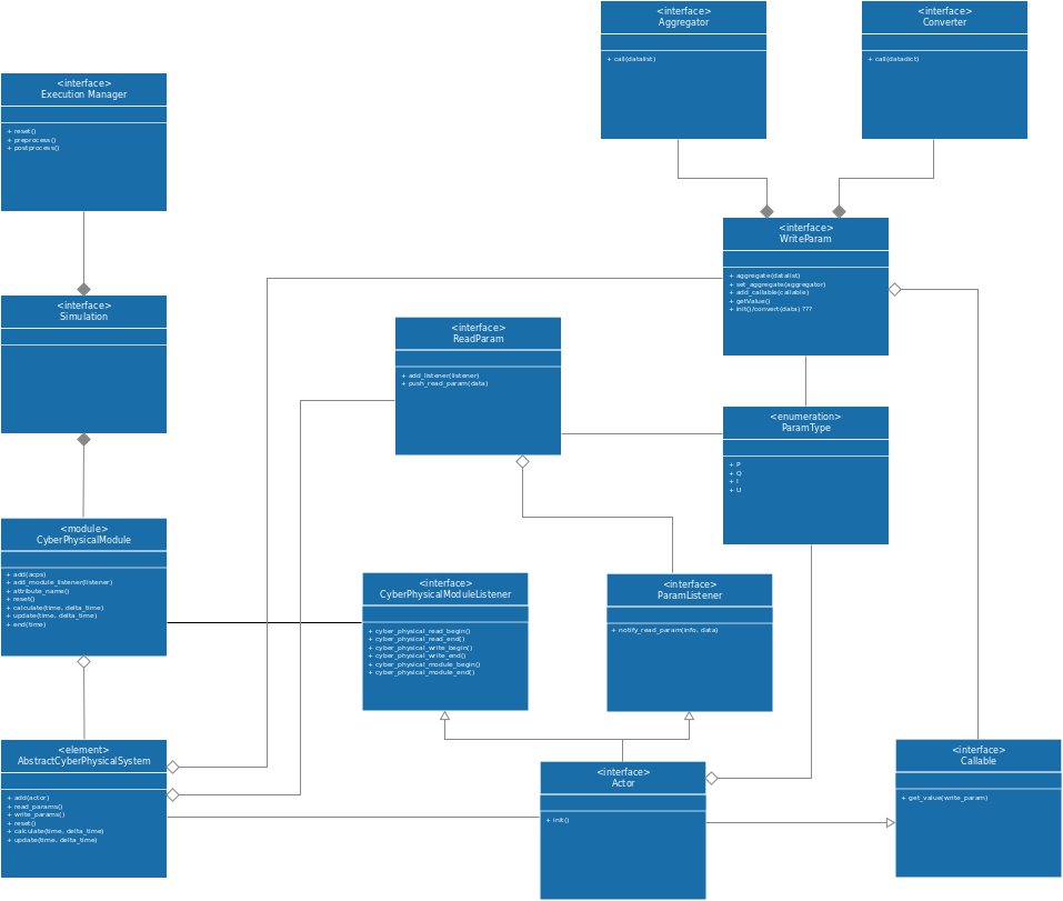
2.1.3.1. Cyber-physical package
Code author: Yann Maret <yann.maret@hevs.ch>
-
class
gridsim.cyberphysical.simulation.CyberPhysicalModuleListener(self)¶ This Listener is informed when the module start an action (read, write) or at the initialisation (
CyberPhysicalModule.reset()) or the end (CyberPhysicalModule.end()) of a step.Warning
This interface does not extend
objectclass. As its implementation should implements another class (e.g.ParamListener), a diamond problem could arise.-
cyberphysical_read_begin(self)¶ Called by the module when the Read begin.
-
cyberphysical_read_end(self)¶ Called by the module when the Read end.
-
cyberphysical_write_begin(self)¶ Called by the module when the Write begin.
-
cyberphysical_write_end(self)¶ Called by the module when the Write end.
-
cyberphysical_module_begin(self)¶ Called by the module when the simulation begin.
-
cyberphysical_module_end(self)¶ Called by the module when the simulation end.
-
-
class
gridsim.cyberphysical.simulation.CyberPhysicalModule(self)¶ Bases:
gridsim.core.AbstractSimulationModuleCyberPhysicalModule registers
AbstractCyberPhysicalSystem(which aregridsim.core.AbstractSimulationElement) and calls :func:`gridsim.core.AbstractSimulationElement.calculateandgridsim.core.AbstractSimulationElement.update()when the simulation is running. It informs all the subscribers, when a Read and Write start and end. This allows easy logging at the end of a cycle.-
add_actor_listener(self, acps)¶ Adds an
gridsim.core.AbstractCyberPhysicalSystemto the module list.Parameters: acps – gridsim.cyberphysical.external.AbstractCyberPhysicalSystemto register the the moduleReturns: the gridsim.cyberphysical.external.AbstractCyberPhysicalSystem.
-
add_module_listener(self, actor)¶ Adds a
CyberPhysicalModuleListenerto the module , calls the listener when the simulation starts, stops, or do an action (read or write).Parameters: listener – CyberPhysicalModuleListenerto notify the status of the simulationReturns: the CyberPhysicalModuleListener
-
attribute_name()¶ attribut_name(self)
Returns the name of this module. This name is used to access to this electrical simulator from the
Simulator:# Create the simulation. sim = Simulator() the_sim = sim.cyberphysical
Returns: ‘cyberphysical’ Return type: str
-
reset()
-
calculate(time, delta_time)
-
update(time, delta_time)
-
end(time)
-
-
class
gridsim.cyberphysical.simulation.MinimalCyberPhysicalModule(self)¶ Bases:
gridsim.core.AbstractSimulationModuleThis module is used to get the update and calculate function from the simulation. This is useful to synchronize an
gridsim.cyberphysical.external.Actorwith the current step (time) of the simulation. This class calls all the listeners and informs them for a step of simulation which include when agridsim.core.AbstractSimulationElement.calculate()andgridsim.core.AbstractSimulationElement.update()functions are called.-
add_element(*args, **keywords)
-
attribute_name()
-
reset()
-
calculate(time, delta_time)
-
update(time, delta_time)
-
2.1.3.2. Cyber-physical elements
Code author: Yann Maret <yann.maret@hevs.ch>
-
class
gridsim.cyberphysical.element.Actor(self)¶ Bases:
gridsim.cyberphysical.core.Callable,gridsim.cyberphysical.core.ParamListenerAn actor represents a (set of) virtual device. Therefore it has to communicate with a real device to send energy to a real network. To do so, it has to be connected to
gridsim.cyberphysical.core.ReadParamto receive data from real device and connected togridsim.cyberphysical.core.WriteParamto influence a device. This is done by a registration to anAbstractCyberPhysicalSystem. This registration also adds theActorto the simulation.Note
More details about
Actorcan be found at The Actors.-
notify_read_param(self, read_param, data)¶ Notifies the listener that a new value from the simulator has been updated.
Parameters: - read_param – paramtype id of the data notified
- data – data updated itself
-
get_value(self, write_param)¶ This function is called by the simulation each time a new value is required with the
write_paramid.Parameters: write_param – The id of the gridsim.cyberphysical.core.WriteParamassociated with the return valueReturns: value that correspond to the given gridsim.cyberphysical.core.WriteParam
-
-
class
gridsim.cyberphysical.element.AbstractCyberPhysicalSystem(self, friendly_name)¶ Bases:
gridsim.core.AbstractSimulationElementAn
AbstractCyberPhysicalSystemcreates ReadParam and WriteParam to communicate with real devices. Actors can be registered to anAbstractCyberPhysicalSystemto influence the real device theAbstractCyberPhysicalSystemis connected.Parameters: - friendly_name – give a friendly name for the element in the simulation
- converters – Dict of Converter function for the write params
-
add(self, actor)¶ Adds an actor to the system and register it with the ReadParam and WriteParam that it wants to be connected.
Parameters: actor – Actorto register in the systemReturns: the Actor
-
physical_read_regulation(*args, **keywords)¶ physical_read_regulation(self, write_param):
This is the measure value for regulator
Returns: read value from physical device
-
physical_read_params(self)¶ Reads the data on the system.
Returns: read data list
-
physical_converter_params(self, write_params)¶ Parameters: write_params – list of data to convert Returns: list of data converted
-
physical_regulation_params(self, write_params)¶ Parameters: write_params – Returns:
-
physical_write_params(self, write_params)¶ Writes the data to the system.
Parameters: write_params – map of {id:datas} to write to the cyberphysical system
-
init_regulator(write_params)
-
regulation()
-
reset(self)¶ Nothing to reset.
2.1.3.3. Cyber-physical aggregator
Code author: Yann Maret <yann.maret@hevs.ch>
-
class
gridsim.cyberphysical.aggregator.SumAggregator(self)¶ Bases:
gridsim.cyberphysical.core.AggregatorSum Aggregator class. This takes all the value and make a simple sum over them and return the result.
-
call(self, data)¶ Aggregate the data with a sum and return the result
Parameters: data – list of data to aggregate, in this case it’s a sum Returns: the sum of the given list value
-
-
class
gridsim.cyberphysical.aggregator.MeanAggregator(self, limit_min, limit_max, default)¶ Bases:
gridsim.cyberphysical.core.AggregatorMean Aggregator class. This does the average value after calling the SumAggregator ‘call’ function
-
call(*args, **keywords)
-
2.1.4. Thermal simulation
The thermal simulation module offers a very abstract thermal simulation. The simulation is based on the thermal capacity of a thermal process (envelope) and the energy flows between those processes via thermal couplings that result as consequence of the temperature differences between the thermal processes and the thermal conductivity of the couplings between them.
Example:
1 2 3 4 5 6 7 8 9 10 11 12 13 14 15 16 17 18 19 20 21 22 23 24 25 26 27 28 29 30 31 32 33 34 35 36 37 38 39 40 41 42 43 44 45 46 47 48 49 50 51 52 | from gridsim.unit import units
from gridsim.simulation import Simulator
from gridsim.recorder import PlotRecorder
from gridsim.thermal.core import ThermalProcess, ThermalCoupling
from gridsim.thermal.element import TimeSeriesThermalProcess
from gridsim.timeseries import SortedConstantStepTimeSeriesObject
from gridsim.iodata.input import CSVReader
from gridsim.iodata.output import FigureSaver, CSVSaver
# Gridsim simulator.
sim = Simulator()
# Create a simple thermal process: A room thermal coupling between the room and
# the outside temperature.
# ___________
# | |
# | room |
# | 20 C | outside <= example time series (CSV) file
# | |]- 3 W/K
# |___________|
#
celsius = units(20, units.degC)
room = sim.thermal.add(ThermalProcess.room('room',
50*units.meter*units.meter,
2.5*units.metre,
units.convert(celsius, units.kelvin)))
outside = sim.thermal.add(
TimeSeriesThermalProcess('outside', SortedConstantStepTimeSeriesObject(CSVReader('./data/example_time_series.csv')),
lambda t: t*units.hours,
temperature_calculator=
lambda t: units.convert(units(t, units.degC), units.kelvin)))
sim.thermal.add(ThermalCoupling('room to outside', 1*units.thermal_conductivity,
room, outside))
# Create a plot recorder that records the temperatures of all thermal processes.
temp = PlotRecorder('temperature', units.second, units.degC)
sim.record(temp, sim.thermal.find(has_attribute='temperature'))
print("Running simulation...")
# Run the simulation for an hour with a resolution of 1 second.
sim.reset(31*4*units.day)
sim.run(31*units.day, 1*units.hours)
print("Saving data...")
# Create a PDF document, add the two figures of the plot recorder to the
# document and close the document.
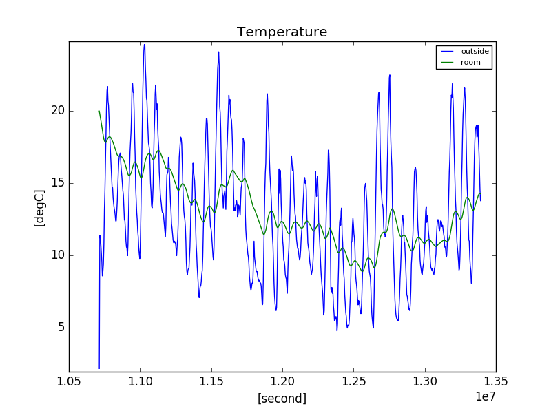
FigureSaver(temp, "Temperature").save('./output/thermal-example.pdf')
FigureSaver(temp, "Temperature").save('./output/thermal-example.png')
CSVSaver(temp).save('./output/thermal-example.csv')
|
- On line 11 we create a new simulation.
- On lines 22 to 35 we create a very simple thermal process with one room and the outside temperature from a data file.
- On line 38 we create a plot recorder and on line 39 we record all temperatures using the plot recorder.
- On line 44 & 45 we initialize the simulation and start the simulation for the month avril with a resolution of 1 hour.
- On linea 51 to 53 we save the data in several formats.
The figure looks like this one:
Here is the class diagram of the thermal package:
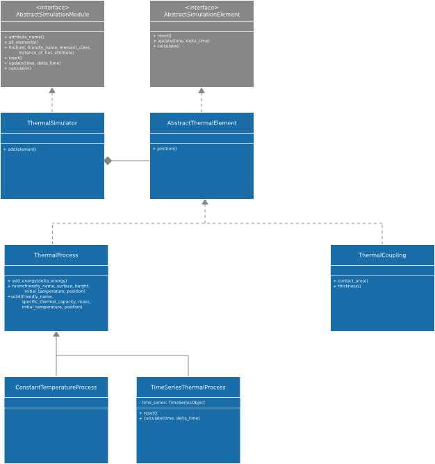
2.1.4.1. Thermal package
-
class
gridsim.thermal.simulation.ThermalSimulator(self)¶ Bases:
gridsim.core.AbstractSimulationModuleGridsim main simulation class for thermal part. This module is automatically added to the
Simulatorwhen importing any class or module ofgridsim.thermalpackage.To access this class from simulation, use
Simulatoras follow:# Create the simulation. sim = Simulator() thsim = sim.thermal
-
attribute_name(self)¶ Returns the name of this module. This name is used to access to this electrical simulator from the
Simulator:# Create the simulation. sim = Simulator() thsim = sim.thermal
Returns: ‘thermal’ Return type: str
-
all_elements(self)¶ Returns a list of all
AbstractThermalElementcontained in the module. The core simulator will use these lists in order to be able to retrieve objects or list of objects by certain criteria usinggridsim.simulation.Simulator.find().Returns: a list of all AbstractThermalElementReturn type: list
-
reset(self)¶ Calls
gridsim.core.AbstractSimulationElement.reset()of each element in this thermal simulator, added by theThermalSimulator.add().
-
calculate(self, time, delta_time)¶ Calls
gridsim.core.AbstractSimulationElement.calculate()of eachThermalProcessin this thermal simulator, added by theThermalSimulator.add()then apply theThermalCouplingto update the energy of each process.Parameters: - time (int or float in second) – The actual simulation time.
- delta_time (int or float in second) – The time period for which the calculation has to be done.
-
update(self, time, delta_time)¶ Updates the data of each
AbstractThermalElementin this electrical simulator added by theThermalSimulator.add()and calculate the load flow withAbstractElectricalLoadFlowCalculator.Parameters: - time (int or float in second) – The actual simulation time.
- delta_time (int or float in second) – The time period for which the calculation has to be done.
-
add(self, element)¶ Adds the
ThermalProcessorThermalCouplingto the thermal simulation module.Parameters: element ( AbstractThermalElement) – Element to add to the thermal simulator module.
-
2.1.4.2. Thermal elements
-
class
gridsim.thermal.element.ConstantTemperatureProcess(self, friendly_name, temperature, position=Position())¶ Bases:
gridsim.thermal.core.ThermalProcessThis is a special thermal process with an infinite thermal capacity which results that the temperature of the process is constant, independent how much energy is taken from or given to the process.
Parameters: - friendly_name (str, unicode) – Friendly name to give to the process.
- temperature (temperature) – The (constant) temperature in degrees celsius.
- position (
Position) – The position of theThermalProcess.
-
add_energy(self, delta_energy)¶ Does nothing at all for this type of
ThermalProcess.
-
update(self, time, delta_time)¶ Does nothing at all for this type of
ThermalProcess.Parameters: - time (float in second) – The actual time of the simulator.
- delta_time (float in second) – The delta time for which the calculation has to be done.
-
class
gridsim.thermal.element.TimeSeriesThermalProcess(self, friendly_name, time_series, stream, time_converter=None, temperature_calculator=lambda t: units.convert(t, units.kelvin), position=Position())¶ Bases:
gridsim.thermal.core.ThermalProcessThermal process that reads the temperature out of a time series object (CSV file). It has an infinite thermal capacity.
Warning
It is important that the given data contains the field ‘temperature’ or you map a field to the attribute ‘temperature’ using the function
gridsim.timeseries.TimeSeriesObject.map_attribute().Parameters: - friendly_name (str, unicode) – Friendly name to give to the process.
- temperature_calculator –
- position (
Position) – The position of the thermal process.
-
reset(self)¶ Sets the time to default (
0).
-
calculate(self, time, delta_time)¶ Calculates the temperature of the element during the simulation step.
Parameters: - time (float in second) – The actual time of the simulator.
- delta_time (float in second) – The delta time for which the calculation has to be done.
-
update(self, time, delta_time)¶ Does nothing for this type of
ThermalProcess.Parameters: - time (float in second) – The actual time of the simulator.
- delta_time (float in second) – The delta time for which the calculation has to be done.
2.2. User Interface
2.2.1. Control of simulation elements
2.2.2. Record of simulation elements
Module author: Michael Clausen <clm@hevs.ch>
Code author: Michael Clausen <clm@hevs.ch>
Code author: Gillian Basso <gillian.basso@hevs.ch>
The gridsim.recorder module allows to record signals within the
gridsim simulation for later analysis. The module offers already a great
number of ready to use recorders - for example to write the data to text or
csv files or to plot the data after the simulation.
However if a special behavior is needed, custom recorders implementing the
Recorder can be implemented.
Here an example illustrating the implementation of a custom recorder and how recorders are added to the simulation:
1 2 3 4 5 6 7 8 9 10 11 12 13 14 15 16 17 18 19 20 21 22 23 24 25 26 27 28 29 30 31 32 33 34 35 36 37 38 39 40 41 42 43 44 45 46 47 48 49 50 51 52 53 54 55 56 57 58 59 | from gridsim.simulation import Simulator
from gridsim.unit import units
from gridsim.recorder import Recorder
from gridsim.thermal.core import ThermalProcess, ThermalCoupling
#Custom recorder.
class ConsoleRecorder(Recorder):
def __init__(self, attribute_name, x_unit, y_unit):
super(ConsoleRecorder, self).__init__(attribute_name, x_unit, y_unit)
def on_simulation_reset(self, subjects):
print 'RESET, observing: ' + str(subjects)
def on_simulation_step(self, time):
# time is given in SI unit (i.e. second)
print 'time = ' + str(units.convert(time*units.second, self._x_unit)) + ':'
def on_observed_value(self, subject, time, value):
# time and value are given in SI unit (i.e. second and kelvin)
print ' ' + subject + '.' + self.attribute_name +\
' = ' + str(units.convert(value*units.kelvin, self._y_unit))
# Create simulator.
sim = Simulator()
# Setup topology (For simplicity we just take a trivial thermal simulation):
# __________ ___________
# | | ___________ | |
# | hot_room |]-----| coupling |-------[| cold_room |
# | 60 C | | 1m2 | | |
# | | |__100_W/K__| | 20 C |
# |__________| <-----------> |___________|
# 1m
celsius = units(60, units.degC)
hot_room = sim.thermal.add(ThermalProcess.room('hot_room',
50*units.meter*units.meter,
2.5*units.metre,
celsius.to(units.kelvin)))
celsius = units(20, units.degC)
cold_room = sim.thermal.add(ThermalProcess.room('cold_room',
50*units.meter*units.meter,
2.5*units.metre,
celsius.to(units.kelvin)))
sim.thermal.add(ThermalCoupling('coupling',
100*units.thermal_conductivity,
hot_room, cold_room))
# Add a custom console recorder to the attribute "temperature" of the hot
# room thermal process.
sim.record(ConsoleRecorder("temperature", units.second, units.degC),
sim.thermal.find(element_class=ThermalProcess))
# Simulate
sim.run(1*units.hour, 5*units.minute)
|
- On lines 8 to 23 we implement our custom recorder.
- On lines 13 & 14 we re-implement the abstract method
gridsim.simulation.Recorder.on_simulation_reset(). We log which objects we observe. - On lines 16 to 18 we implement the
gridsim.simulation.Recorder.on_simulation_step()method. We just output the current time. The time is given in a float in second. - On lines 20 to 23 we re-implement the abstract method
gridsim.simulation.Recorder.on_observed_value(). Basically we just output the value to the console. The time is given in a float in second.
- On lines 13 & 14 we re-implement the abstract method
- On line 26 we create the gridsim simulation object.
- On lines 37 to 51 we setup a very simple thermal process, where we define 2
rooms and a thermal coupling between them:
- hot_room (line 38) has a
surfaceof50m2and aheightof2.5m, so thevolumeis125m3. The room is filled withgridsim.util.Air(specific thermal capacity=`1005 J/kgK``) with the initial temperature of 60 degree celsius (line 38). - cold_room (line 44) has the same volume, but an initial temperature of 20 degree celsius (line 43).
- the two rooms are coupled with a thermal conductivity of
100 Watts per
Kelvin
(lines 49 to 51).
- hot_room (line 38) has a
- On lines 55 & 56 we add the recorder to the simulation. The recorder will
listen all
ThermalProcessand record theirtemperatureparameter. The horizontal unit will be in second and the vertical unit in degree celsius. The simulation will call the recorder’s on_simulation_step() and on_observed_value() method each time the simulation did a step. - On line 59 we actually start the simulation for 1 hour with a resolution of 5 minutes.
The output of the console logger should be something like this:
RESET, observing: ['hot_room', 'cold_room']
time = 0 second:
    hot_room.temperature = 60.0 degC
    cold_room.temperature = 20.0 degC
time = 300.0 second:
    hot_room.temperature = 52.039800995 degC
    cold_room.temperature = 27.960199005 degC
time = 600.0 second:
    hot_room.temperature = 47.2478404 degC
    cold_room.temperature = 32.7521596 degC
time = 900.0 second:
    hot_room.temperature = 44.363127803 degC
    cold_room.temperature = 35.636872197 degC
time = 1200.0 second:
    hot_room.temperature = 42.6265595232 degC
    cold_room.temperature = 37.3734404768 degC
time = 1500.0 second:
    hot_room.temperature = 41.581162698 degC
    cold_room.temperature = 38.418837302 degC
time = 1800.0 second:
    hot_room.temperature = 40.9518442113 degC
    cold_room.temperature = 39.0481557887 degC
time = 2100.0 second:
    hot_room.temperature = 40.5730007441 degC
    cold_room.temperature = 39.4269992559 degC
time = 2400.0 second:
    hot_room.temperature = 40.3449407464 degC
    cold_room.temperature = 39.6550592536 degC
time = 2700.0 second:
    hot_room.temperature = 40.2076508971 degC
    cold_room.temperature = 39.7923491029 degC
time = 3000.0 second:
    hot_room.temperature = 40.1250037739 degC
    cold_room.temperature = 39.8749962261 degC
time = 3300.0 second:
    hot_room.temperature = 40.0752510281 degC
    cold_room.temperature = 39.9247489719 degC
time = 3600.0 second:
    hot_room.temperature = 40.0453003701 degC
    cold_room.temperature = 39.9546996299 degC
-
class
gridsim.recorder.PlotRecorder(self, attribute_name, x_unit=None, y_unit=None)¶ Bases:
gridsim.simulation.Recorder,gridsim.iodata.output.AttributesGetterA
PlotRecordercan be used to record one or multiple signals and plot them at the end of the simulation either to a image file, add them to a PDF or show them on a window.Parameters: - attribute_name (str) – The attribute name to observe. Every
AbstractSimulationElementwith a param of this name can be recorded - x_unit (int, float, type or unit see
gridsim.unit) – The unit of the horizontal axis - y_unit (int, float, type or unit see
gridsim.unit) – The unit of the vertical axis
If no information are give to the constructor of a
Recorder, the data are not preprocessed.Warning
The preprocess can take a long time if a lot of data are stored in a
PlotRecorder.Example:
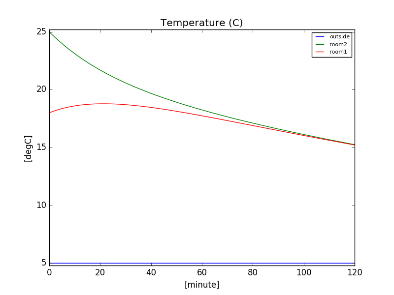
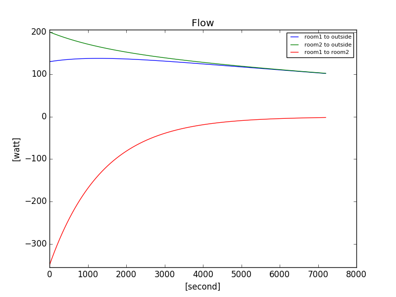
 1
 2
 3
 4
 5
 6
 7
 8
 9
10
11
12
13
14
15
16
17
18
19
20
21
22
23
24
25
26
27
28
29
30
31
32
33
34
35
36
37
38
39
40
41
42
43
44
45
46
47
48
49
50
51
52
53
54
55
56
57
58
59
60
61
62
63
64
65
66
67
68
69
70
71
72
from gridsim.unit import units
from gridsim.simulation import Simulator
from gridsim.thermal.core import ThermalCoupling, ThermalProcess
from gridsim.thermal.element import ConstantTemperatureProcess
from gridsim.recorder import PlotRecorder
from gridsim.iodata.output import FigureSaver, CSVSaver

# Gridsim simulator.
sim = Simulator()

# Create a simple thermal process: Two rooms and the thermal coupling between
# them and to the outside temperature.
#             __________                        ___________
#           |          |   ________________   |           |
#           |   room1  |]-| room1 to room2 |-[| cold_room |
#           |    18 C  |  |_____50_W/K_____|  |    25 C   |      outside 5 C
#  10 W/K -[|          |                      |           |]- 10 W/K
#           |__________|                      |___________|
#
celsius = units(18, units.degC)
room1 = sim.thermal.add(ThermalProcess.room('room1',
                                            50*units.meter*units.meter,
                                            2.5*units.metre,
                                            units.convert(celsius, units.kelvin)))
celsius = units(25, units.degC)
room2 = sim.thermal.add(ThermalProcess.room('room2',
                                            50*units.meter*units.meter,
                                            2.5*units.metre,
                                            units.convert(celsius, units.kelvin)))

celsius = units(5, units.degC)
outside = sim.thermal.add(
    ConstantTemperatureProcess('outside', units.convert(celsius, units.kelvin)))

sim.thermal.add(ThermalCoupling('room1 to outside',
                                10*units.thermal_conductivity,
                                room1, outside))
sim.thermal.add(ThermalCoupling('room2 to outside',
                                10*units.thermal_conductivity,
                                room2, outside))
sim.thermal.add(ThermalCoupling('room1 to room2',
                                50*units.thermal_conductivity,
                                room1, room2))

# Create a plot recorder that records the temperatures of all thermal processes.
kelvin = PlotRecorder('temperature', units.second, units.kelvin)
sim.record(kelvin, sim.thermal.find(has_attribute='temperature'))

# Create a plot recorder that records the temperatures of all thermal
# processes in Kelvin.
celsius = PlotRecorder('temperature', units.minutes, units.degC)
sim.record(celsius, sim.thermal.find(has_attribute='temperature'))

# Create a second plot recorder which records all energy flows
# (thermal couplings) between the different processes.

flow = PlotRecorder('power', units.second, units.watt)
sim.record(flow, sim.thermal.find(element_class=ThermalCoupling))

print("Running simulation...")

# Run the simulation for an hour with a resolution of 1 second.
sim.run(2*units.hour, 1*units.second)

print("Saving data...")

# Save the figures as images.
FigureSaver(kelvin, "Temperature (K)").save('./output/fig1.png')
FigureSaver(celsius, "Temperature (C)").save('./output/fig2.png')
FigureSaver(flow, "Flow").save('./output/fig3.png')

CSVSaver(celsius).save('./output/fig2.csv')
- In this example, only new concept are detailed.
- On line 46, we create a
PlotRecorderwhich recorder thetemperatureattribute in Kelvin. - On line 47, we use that recorder in order to record all element in
the thermal module who have the attribute ‘temperature’ by using the
powerful
gridsim.simulation.Simulator.find()method by asking to return a list of all element that have the attribute ‘temperature’. - On line 51, we create a very similar recorder as before, but the attribute will be in celsius and the time in minutes.
- On line 52, we recorder same objects as above,
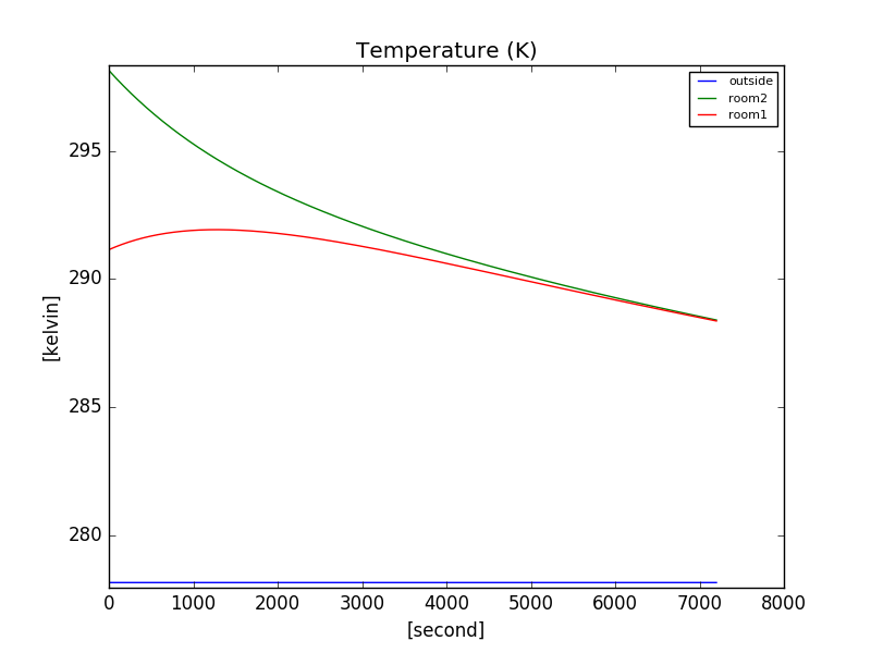
- On line 68, we create a first
FigureSaverinstance with the title ‘Temperature (K)’ which will use the data returned by theRecordertosave()the data in a figure. - On line 69, we also save the data of the other
Recorder. The figures below show that the result is quite the same except that the y-coordinates have the right unit. - On line 72, we save the data using another saver:
CSVSaver.
The resulting 3 images of this simulation are show here:
-
on_simulation_reset(self, subjects)¶ Recorderimplementation. Prepares the data structures.See also
gridsim.simulation.Recorder.on_simulation_reset()for details.
-
on_simulation_step(self, time)¶ Recorderimplementation. Prepares the data structures.See also
gridsim.simulation.Recorder.on_simulation_step()for details.
-
on_observed_value(self, subject, time, value)¶ Recorderimplementation. Saves the data in order to plot them afterwards.See also
gridsim.simulation.Recorder.on_observed_value()for details.
-
x_values(self)¶ Retrieves a list of time, on for each
on_observed_value()and ordered following the call ofgridsim.simulation.Simulator.step().Example:
sim = Simulator()

kelvin = PlotRecorder('temperature')
sim.record(kelvin, sim.thermal.find(has_attribute='temperature'))

sim.step(17*units.second)
sim.step(5*units.second)
sim.step(42*units.second)
In this example, this function should returns:
[17, 5, 42]
Returns: time in second Return type: list
-
x_unit(self)¶ Retrieves the unit of the time.
Returns: the time unit, see gridsim.unitReturn type: str
-
y_values(self)¶ Retrieves a map of the recorded data:
{
    id1: [list of recorded values]
    id2: [list of recorded values]
}
with
idXthesubjectgiven in parameter ofon_observed_value()andon_simulation_reset()Returns: a map associating id to recorded data Return type: dict
-
y_unit(self)¶ Retrieves the unit od the recorded data.
Returns: the type or the unit, see gridsim.unitReturn type: str
- attribute_name (str) – The attribute name to observe. Every
-
class
gridsim.recorder.HistogramRecorder(*args, **keywords)¶ Bases:
gridsim.simulation.Recorder,gridsim.iodata.output.AttributesGetterWarning
This class is currently not tested...
Parameters: - attribute_name –
- x_min –
- x_max –
- nb_bins –
- x_unit (type or unit see
gridsim.unit) – The unit of the horizontal axis - y_unit (type) – The unit of the vertical axis
Returns: -
on_simulation_reset(subjects)¶ RecorderInterfaceimplementation. Writes the header to the file defined by the _header_format attribute each time the simulation does a reset.See also
RecorderInterface.on_simulation_reset()for details.
-
on_simulation_step(time)¶ RecorderInterfaceimplementation. Called for each simulation step once per recorder. Writes the step separation to the file.See also
RecorderInterface.on_simulation_step()for details.
-
on_observed_value(subject, time, value)¶ RecorderInterfaceimplementation. Writes a (formatted) string into the file.See also
RecorderInterface.on_observed_value()for details.
-
x_values()
-
x_unit(*args, **keywords)
-
y_values()
-
y_unit(*args, **keywords)